
Natural Selection Simulator Analysis
View on GitHub 
View Simulator development page
Summary
There is an attached Jupyter notebook, summary.ipynb, which has various methods for reading CSV files into Pandas dataframes and plotting relevant statistics. For example the average attributes of noodles by timestep, showing how the population evolves over time:
The variability in random starting populations and immigration means that several simulations can be drastically different even if the values such as environment size, food density, and starting population remain constant.
Populations usually converge to the set of attributes with the highest fitness for that specific population. So, while one set of attributes may be best to compete for resources against a random selection of other noodles, a more efficient set of attributes may be needed to compete against similar noodles.
Examples without Predators
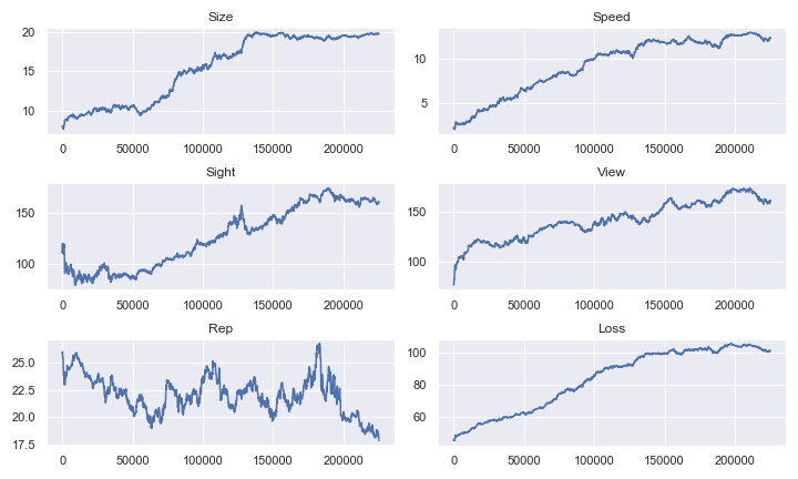
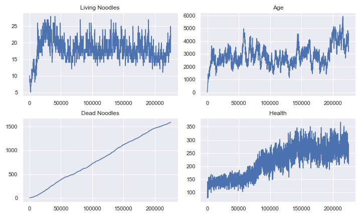
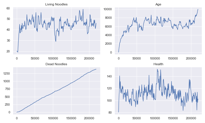
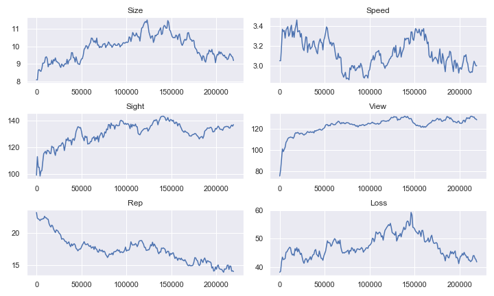
An example simulation without predators shows how the population evolves to increase all of their attributes and loss. The more efficient noodles are also longer living as they evolve, shown in the average age of noodles towards the end, and their reproduction rate is selected as a necessarily beneficial trait.
The populations’ size, average age, total deaths, and average health over time:
The populations’ average attributes:
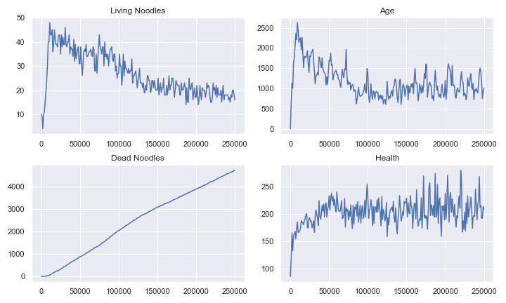
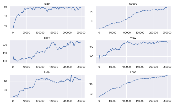
The same exact settings can have a very different outcome, showing the potential diversity. This simulation’s noodles ended up evolving to favor fast reproducing noodles with short lifespans. Their average age is around 1/4 of the previous example, but their reproduction rate has been genetically selected by the environment with an average rate 4 times the previous population’s. Their attributes and loss are still increasing, showing how they still evolve to be competitive and towards higher fitness, but with the aim to reproduce quickly instead of living long enough to reproduce.
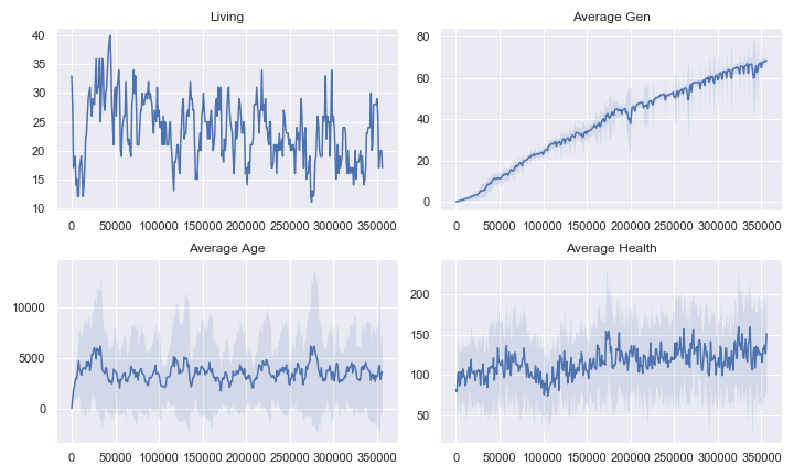
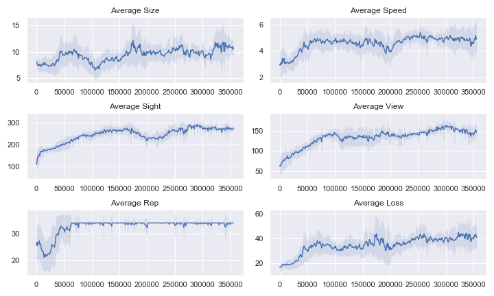
When the environment is expanded and the abundance of food is increased, a larger population forms. These noodles are also living much longer, but with less competitive attributes such as speed and sight. Speed may not be worth the compensation in loss if there is more food around, and sight isn’t as important with shorter distances to food. Longer sight ranges may even be detrimental, since the noodle will go for the first food it sees, not the closest. In an environment with more noodles to compete with, it may be beaten to the food more easily.
Over time you can see how attributes converge in a population. In this example reproduction doesn’t have a change to mutate, with the other attributes converging despite fluctuations in population size, with a relatively low loss selected for. The average generation of the noodles at the end is over 60, and the standard deviations can also be seen in light blue around the averages in the graphs.
Examples with Predators
Observing the interaction between preds and noodles is very interesting. This example shows how the populations depend on each other: a large starting noodle population means an abundance of food for predators, who quickly deplete their food source and keep their own population in check. The fluctuation in populations continues in a cycle, with more prey allowing more predators to exist, but the greater number of predators quickly eating up all the prey.
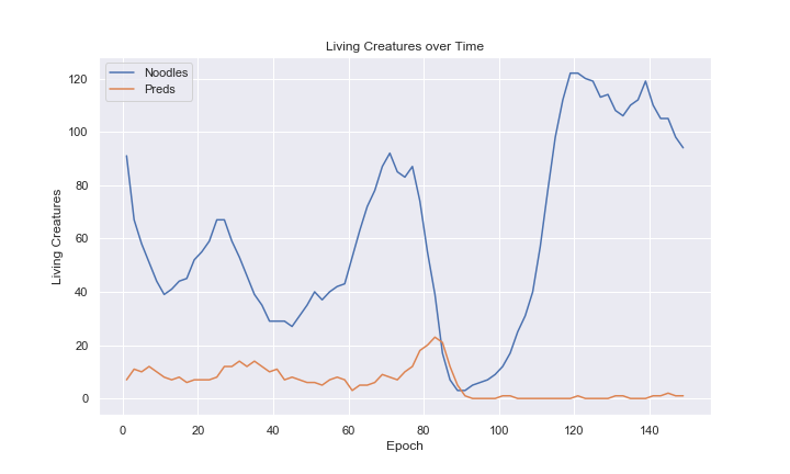
A large influx of predators around epoch 80 quickly decimates the noodle population and the scarcity of food finishes off the predators. The noodle population recovers, but immigrating predators are unable to establish a foothold in the new noodle population, where the noodles are much faster now and reproduce more quickly.
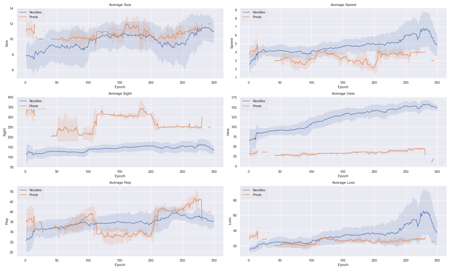
This cycle can play out several times, seen in this simulation which fluctuating cycles but also eras of stability.
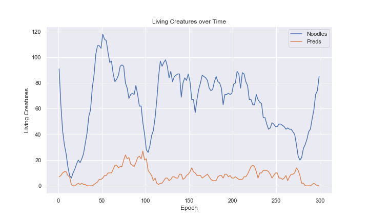
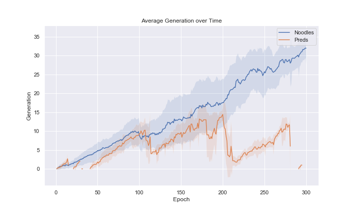
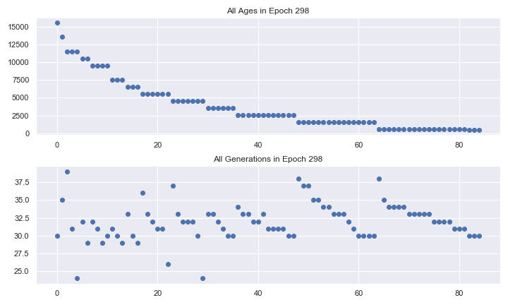
After epoch 100 when a large number of noodles and predators die off, there is a stable period. This is likely due to more predators coming from a common ancestor. This can be seen by looking at the average generations which shows a dropoff after epoch 100, indicating more creatures in that population are offspring of a new species, instead of the starting species.
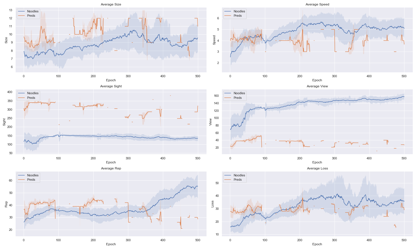
This predator species is characterized by being slower with a longer range of vision and lesser reproduction rate. These creatures are actually slower than their average prey but can see far enough that they are able to eat enough to survive. They don’t frequently reproduce, which limits the chance of a population explosion that would decimate their prey. The noodles eventually get too fast for them though, and they aren’t able to survive anymore.
Other tools in the summary notebook allow for exploring statistics of individual epochs. Age and generation of each living noodle in the 298th epoch can be viewed:
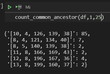
Common ancestors’ attributes can be viewed by epoch, showing over 80 living noodles who came from the same set of attributes in the 25th to last epoch. Just a few of the noodles came from ancestors who were much bigger, faster, and with better vision:
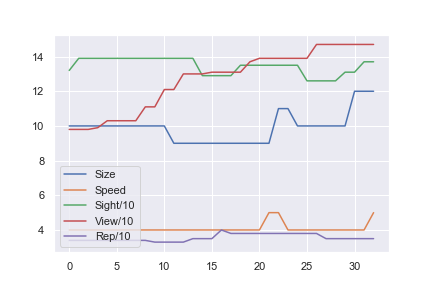
And each noodle can be selected to see how their traits have changed over time through their ancestry tree:
These are just a few examples which have CSVs in data, but there are countless other simulations showing all sorts of evolution and interaction between species, with lots of interesting insights and sometimes hard to explain phenomena thanks to the intentional randomness.